Our funding comes from our readers, and we may earn a commission if you make a purchase through the links on our website.
Traffic Shaping – What is It and How-TO Guide (Configuration & Monitoring)
UPDATED: March 27, 2023
Have you ever been on a network where some applications (going over the Internet) are slower than others? A typical example is companies that slow down (or restrict completely) the speed of torrent applications –
This is Called Traffic Shaping.
This is usually done to discourage users of that network from using those kinds of applications, maybe during certain hours, because the use of such applications can affect the service of other users on the network.
Note: Many torrent applications now encrypt their traffic making it more difficult to identify those kinds of application and applying any sort of traffic policy on them.
Generally speaking, there are four factors that affect the quality of a Network:
- Bandwidth
- Delay
- Internet Jitter
- Packet Loss
In a network where all devices are in close proximity to each other and where bandwidth is not a problem (e.g. a Local Area Network), these four factors may not be too much of an issue. In such networks, you just need to make sure your cables (or wireless connections) have enough capacity to carry the traffic flowing on the network.
The cost of building such a network is typically one-off and not so high.
However, when we get to networks that are far from each other and that need to be connected together (e.g. a Wide Area Network), or connection to a public network like the Internet, then one must pay attention to these network quality factors.
This is because the infrastructure needed to connect to a private WAN or public network is expensive and you typically get what you pay for. In most cases, the cost is also recurring as you need to go through a service provider.
Quality of Service
This brings us to an important question: how do we ensure the quality performance of a network even in cases where connectivity can be expensive? Enter the world of Quality of Service (QoS). Since different applications react differently to the four factors that affect network quality, QoS aims to provide the best level of service for the various types of applications (depending on user requirement).
Let’s take Voice as an example. Even though the packets that make up a voice traffic do not need a lot of bandwidth, voice does not do well with delay and packet loss. You may have noticed this on a voice call using a not-so-good wireless network – lagging is noticeable on such calls and in some cases, you don’t even hear the person on the other end.
On the other hand, when downloading a large file over a TCP connection, bandwidth is the most important factor; TCP can make up for packet loss by retransmitting packets.
For QoS to be implemented properly on a network, there are at least three things to think about:
- Classification of Traffic:
An organization must think about the types of traffic/application running on their network so that they can apply policies to the different classes of traffic. This will typically involve the organization identifying what traffic is critical to their business (e.g. traffic to/from an application server) and defining how such traffic will be matched.In the case of an ISP, they can classify traffic on a per-user basis, per application, etc. Examples of classification methods on Cisco devices include Access Control Lists (ACLs), Committed Access Rate (CAR), and Network-Based Application Recognition (NBAR). - Marking:
When traffic has been classified, some sort of tag may be applied to that traffic so that all devices in the path of the traffic can apply policies (if required) to that traffic. Moreover, relying on common “tags” allows device manufacturers to build default profiles for various classes of traffic.Some of the ways traffic can be marked include using the Differentiated Services Code Points (DSCP) bits, MPLS Experimental bits, IP Precedence (IPP) bits, and so on. - QoS Policies:
The whole point of classifying packets and marking them is so that something can be done to those packets.This means that policies must be applied to marked traffic and when talking about QoS, some of these policies include Congestion Management (e.g. Queuing), Congestion Avoidance (e.g. Weighted Random Early Detection), Traffic Shaping, and Traffic Policing.
Traffic Shaping
We have now come to the focus of this article which is Traffic Shaping. When you hear the word “shaping”, what comes to mind? For me, I think of someone molding a sculpture using clay. The sculptor is able to shape the clay into any form he/she wants.
This is exactly what Traffic Shaping is – the ability to shape a certain category of traffic into a particular form, usually done by controlling the speed of the traffic flow. This means that if the traffic subject to shaping is arriving at a rate lower than the configured rate, then there is no problem – it will be forwarded normally.
However, if the traffic is arriving faster than the configured rate, then it will usually be held in a buffer and delayed until it can be sent out without going over the configured rate.
Note: This is the difference between traffic policing and traffic shaping. In the case of excess traffic flow, traffic policing will usually drop the excess packets while traffic shaping will delay it and send it out at a later time.
Why will you want to implement traffic shaping? Imagine that you are getting Internet from an ISP that has guaranteed you a bandwidth of 2Mbps. Now, the physical link between you and the ISP could be a FastEthernet cable which has a theoretical speed of 100Mbps. This means that theoretically, you can push 100Mbps over that link while paying for only 2Mbps.
So how will the ISP prevent this? Usually, they will implement some form of traffic policing that drops any traffic above the agreed rate (2Mbps). To make sure you are not sending more traffic than the ISP is willing to receive, you can implement traffic shaping on your end such that your traffic will be sent at an average rate of 2Mbps, reducing the chances of the ISP dropping your traffic.
Cisco’s Implementation of Traffic Shaping
The general concept of Traffic Shaping remains the same:
Delay Traffic so that it does not go over a Configured Rate.
Different device manufacturers will implement this feature differently but let us look at how it is implemented on Cisco devices which are very common in enterprise networks.
Cisco’s implementation of Traffic Shaping uses a Token Bucket Metaphor. It is easier to explain this using an example. Imagine a router connected to an ISP via an interface that is capable of sending 10Mbps (i.e. Ethernet).
This means that every second, this interface is capable of sending out about 10,000,000 bits of data.
Now, let us imagine you that the ISP has agreed to give you 2Mbps bandwidth over that Ethernet link. This means that anything extra that you send over 2Mbps will be dropped.
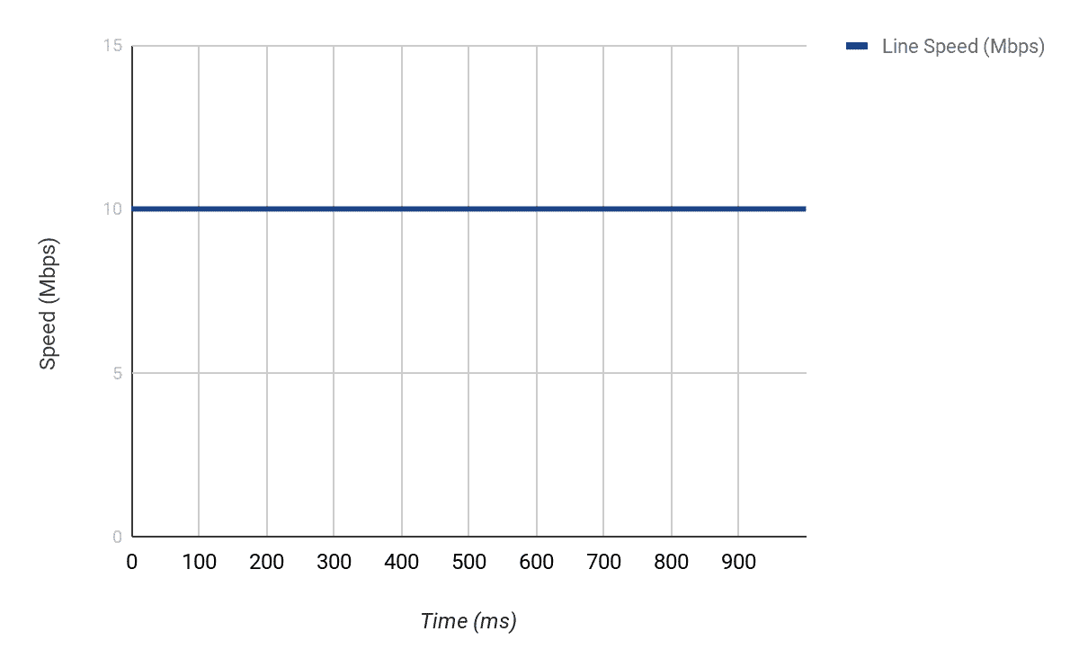
First of all, you must be aware that it is not possible to make an interface send lower than its line speed (in this case, 10Mbps). We cannot physically slow down bits as they exit an interface. So for example:
- If 10 megabits of data are available on an interface, it will take the interface 1 second to send the traffic out i.e. (10 megabits/10 megabits) * 1sec = 1 second.
- If 1 megabits of data is available, it will take the interface (1 megabits/10 megabits) * 1sec i.e. 0.1 second to send out the data.
- If 25 megabits of data are available to be sent out on an interface, it will take the interface (25 megabits/10 megabits) * 1sec = 2.5 seconds.
You should get the point by now, even though this explanation is theoretical. In reality, different factors can affect how quickly packets are sent out an interface, plus the fact that the theoretical speeds of interfaces are not met in practice.
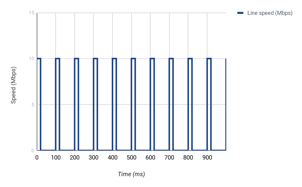
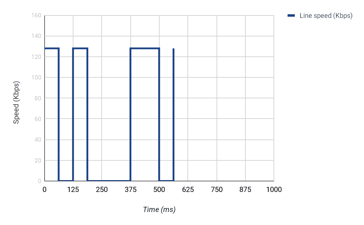
So what can we do? Well, we can make sure only 2Mbps of data (on average) is sent out over the 10Mbps link by delaying packets over a certain interval. In this case, we need to make sure that only 1/5th of the line speed is used in one second i.e. 2Mbps/10Mbps. This will resemble a start-stop operation where we start sending data, stop for a while, send again, and so on.
To conceptualize this, let us divide our 1 second into say 10 parts, which will mean that each part is 100ms (i.e. 100ms * 10 = 1000ms = 1 sec). The problem we then need to solve is, how many bits can we send in each 100ms interval (at a maximum line rate of 10Mbps) to make sure that we only send 2Mbps?
Since we are working with 10 intervals in 1 second, and we need to send 2,000,000 bits per second, it means we need to send 2,000,000 bits/10 every interval i.e. 200,000 bits every 100ms interval.
However, the interface can normally send 1,000,000 bits every 100ms interval (i.e. 10,000,000 bits/10). This means that to be able to send 200,000 bits in a particular interval, we must only send for 20ms [(200,000/1,000,000)*100ms] and then stop for the next 80ms. If we do this 10 times, we will have successfully sent just 2,000,000 bits in one second i.e. 2Mbps.
We will take another example to drive home the point but before we do that, let me introduce the technical terms used when discussing Traffic Shaping:
- Committed Information Rate (CIR):
This is the average speed we want to achieve. From our example, the CIR is 2Mbps or 2,000,000bps - Burst size (Bc):
Also known as Committed Burst size, this is how many bits can be sent per time interval to maintain the CIR. Another way to say it is the Bc is how many tokens (bits) that can be put in the token bucket every time interval. In our example, this is 200,000 bits. - Time Interval (Tc):
This is the measurement interval of how often tokens can be put in the token bucket. In our example, the Tc is 100ms.
Let’s take Another Example:
Imagine that an interface has a line speed of 128Kbps. This means that 128,000 bits can be sent on that interface every second.
Now let us imagine that we want to shape the traffic on that interface to 64Kbps.
This means that our CIR = 64,000bps.
If we divide the token bucket into 8 intervals, for example, it means our Tc = 125ms (i.e. 1second/8). This means that for us to maintain an average rate of 64,000bps over 8 intervals, we need to put 8,000 bits every Tc time interval (i.e. 64,000/8).
From this calculation, a Formula is Evident:
CIR (bps) = Burst size (bits) / Time interval (seconds)
So in this example, we could have also calculated our burst size as CIR * Time interval i.e. (64000 * 0.125) = 8000 bits. This means that every 0.125 second or 125ms, we need to send 8000 bits.
Note: All these equations can be very confusing because they use different units. For example, time interval is usually expressed in ms but when used for calculations, you must convert to seconds. Keep that in mind.
However, the normal line speed of the interface in the example is 128,000 bps. This means that we can normally send 16,000 every 125ms (128,000 * 0.125). Therefore, for us to achieve the CIR we want, we can only send every [(8000/16000) * 125ms] i.e. 62.5ms.

What happens if we don’t use all the Bc during a particular Tc? Well, we can accumulate it and use it during another Tc. For example, if in Tc2 we send 8000 bits but we don’t have any data to send in Tc3, we can use that extra we have saved say during Tc4 which means we can send 8000 (Bc) + 8000 (saved) i.e. 16,000 bits. That extra is known as Excess Burst (Be).
Lab: Traffic Shaping on Cisco routers
All this talk of bits and milliseconds can be very confusing but the implementation is quite simple. In most cases, the only thing you need to decide is your CIR; the Cisco router will calculate the best burst size to use, and with those two values, will determine the correct time interval.
However, there are cases where you want to be specific. For example, for delay sensitive traffic like voice, you may want to use a smaller Tc. By specifying the CIR and burst size, you can change the time interval.
To configure Class-Based Traffic Shaping on a Cisco router, you should:
- Define the traffic you want to shape e.g. using an ACL
- Create a Class Map and match the traffic to be shaped
- Create a Policy Map
- Configure shaping for the class map defined in step 2.
- Apply configured policy map to appropriate interface in the outbound direction
You can skip steps 1 and 2 if you want to shape all traffic going out a particular by using the default “class-default” class map available on Cisco routers. Also, keep in mind that you can only configure shaping in the outbound direction on an interface.
Let’s look at a lab scenario to see how this is done. The lab setup is as shown below:

Let us assume that the bandwidth agreement between the company and the ISP is 8Kbps. As such, the ISP has configured traffic policing on their ISP_RTR. The configuration on that ISP_RTR is as follows:
ip access-list extended CUST_ACL

permit ip 10.1.1.0 0.0.0.255 any

!

class-map match-all CUST_CMAP

match access-group name CUST_ACL

!

policy-map CUST_PMAP

class CUST_CMAP

police 8000 3000

!

interface FastEthernet0/0

Description *** TO SERVER ***

ip address 10.2.2.1 255.255.255.0

!

interface FastEthernet0/1

Description *** TO CUSTOMER ***

ip address 192.0.2.1 255.255.255.0

service-policy input CUST_PMAP

!

ip route 10.1.1.0 255.255.255.0 192.0.2.2
In the configuration above, all traffic from the customer network (10.1.1.0/24) is policed to a rate of 8000bps (8Kbps) with a normal burst size of 3000 bytes.
Note: The CIR and burst size as used in policing is a bit different from how it is used in traffic shaping. The explanation is beyond the scope of this article.
We can take a look at the output of the show policy-map interface command on the ISP_RTR to see the current state of the policing. As we have not sent any traffic, everything will read 0.

Now, let us jump on INSIDE_RTR and try to ping SERVER. This traffic will flow through COMPANY_EDGE to ISP_RTR and then to SERVER (and back). We will increase the size of our ping packets from the default 100 bytes to 500 bytes just so we can hit the policing rate.

Note: You can also perform the same test on PC1 using the following command: ping 10.2.2.100 -l 500 -c 100 -i 200
As you can see, of the 100 packets that were sent, only 80 packets were successful (although some were lost at the beginning due to ARP). Also, notice that the average round-trip time is 98ms. This information is useful to us later on in this article.
If we look at the output of the show policy-map interface command again, we see why those packets were dropped:
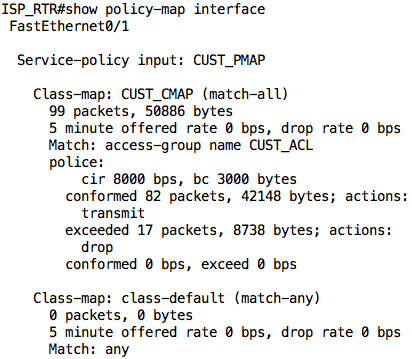
The ISP_RTR dropped 17 of the 99 packets that were sent by INSIDE_RTR.
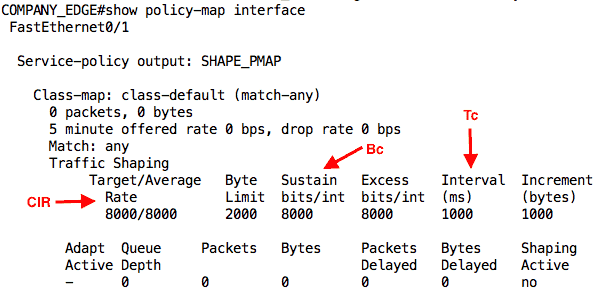
To avoid this issue (to an extent), we can configure traffic shaping on COMPANY_EDGE. The full configuration on that router is as follows:
policy-map SHAPE_PMAP

class class-default

shape average 8000

!

interface FastEthernet0/0

description *** TO LAN ***

ip address 10.1.1.1 255.255.255.0

!

interface FastEthernet0/1

description *** TO ISP ***

ip address 192.0.2.2 255.255.255.0

service-policy output SHAPE_PMAP

!

ip route 10.2.2.0 255.255.255.0 192.0.2.1
In this configuration, we are shaping all traffic (matched in the class-default class-map) to an average rate (CIR) of 8000bps.
Note: In practice, you want your shaper to take effect before you hit the bandwidth limit. A good rule of thumb will be to shape at an average rate of 80-85% of the agreed rate.
We can also use the show policy-map interface command on this router to see the status of our shaping:
Note: Because you matched the default class-map, your output may show that some packets have passed through the interface even before the ping.
With this configuration, let us initiate our ping from INSIDE_RTR to SERVER again:
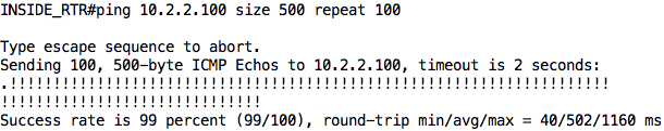
Aha! 99% success rate. The one packet that failed was due to ARP. However, look at the average round-trip time now; it has gone up to 502ms. This already tells us that some packets were delayed by the shaper. We can confirm this from the output of the show policy-map interface command:
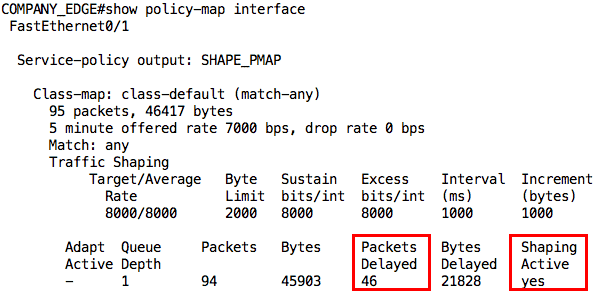
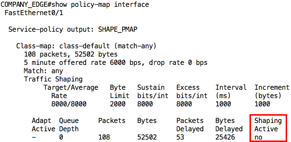
This first output was taken while the ping was still going on. Notice that it says “yes” for Shaping Active. After the ping traffic, the output is slightly different not only in the number of packets delayed but also that shaping is no longer active:
Conclusion
This brings us to the end of this article where we have looked at Traffic Shaping. We discussed why you may want to implement traffic shaping on your network and saw how it can be configured and monitored on Cisco routers.
In our lab, we only looked at Class-Based Traffic Shaping. However, there are other types of traffic shaping like Generic Traffic Shaping, Frame Relay Traffic Shaping, and so on.
Traffic Shaping FAQs
How does traffic shaping enhance network security?
Traffic shaping can enhance network security by limiting the bandwidth used by potentially malicious network traffic, such as spam or malware.
How is traffic shaping configured?
Traffic shaping is typically configured using network management software or specialized traffic shaping devices.
Can traffic shaping be performed on a per-user basis?
Yes, traffic shaping can be performed on a per-user basis, allowing administrators to control the bandwidth used by specific users or groups.
What is the difference between traffic shaping and traffic management?
Traffic shaping is a specific type of traffic management that focuses on controlling and managing the flow of network traffic, while traffic management encompasses a broader range of network management tasks.
What is the difference between traffic shaping and Quality of Service (QoS)?
Traffic shaping and Quality of Service (QoS) are similar in that they both aim to control and manage network traffic, but QoS focuses on prioritizing certain types of traffic, while traffic shaping also includes the ability to limit the bandwidth used by other types of traffic.
Can traffic shaping be used in conjunction with other network management techniques?
Yes, traffic shaping can be used in conjunction with other network management techniques, such as load balancing and network security measures, to provide a comprehensive network management solution.
What are the limitations of traffic shaping?
The limitations of traffic shaping include the need for accurate network information and the potential for network security breaches.